Enhancing Card Sorting Dendrograms through the Holistic Analysis of Distance Methods and Linkage Criteria

Abstract

Card sorting has been widely used in information architecture to analyze and improve web content and navigation. This is an intuitive and cost-effective technique also useful in user research and evaluation. However, while the implementation of sorting tasks comprises a constructive and easy-to-accomplish process, the quantitative analysis of resulting card-sorting data can be a challenge for non-skilled evaluators. Several tools exist to support sorting tasks and data analysis, but still some users utilize custom spreadsheets or statistical packages in order to enhance analysis and obtain more expressive and comparable results.

One of the most utilized diagrams for analyzing card-sorting results is the dendrogram, also known as a tree diagram, which is commonly based on an agglomerative clustering representation depicting groupings of related cards. However, several issues have to be considered by evaluators in order to produce meaningful dendrograms for decision-making. In fact, the distance method and the linkage criterion greatly influence the final dendrogram obtained.

In this paper, an analysis on distance methods and linkage criteria for obtaining suitable dendrograms is proposed. The main aim is to guide evaluators and usability engineers to produce appropriate dendrograms based on available card-sorting data. In this sense, the provided clues can be widely applied to any card-sorting domain and sample size, improving card-sorting analysis by comparing different solutions through goodness indicators.

Analyses applied to a publicly available dataset indicate that the results are highly dependent of the data type, so the right selection of both distance method and linkage criterion is essential for obtaining a suitable dendrogram and correctly interpreting the results.

Keywords

Information architecture, card sorting, quantitative analysis, agglomerative clustering, distance method, linkage criterion, dendrogram

Introduction

Card sorting is a widespread technique that has been used in different domains that range from social sciences to software development (Hudson, 2014). In fact, it has been successfully applied to analyze and improve the information architecture of a website (Rosenfeld & Morville, 2002) through a user-centered approach (Cayola & Macías, 2018; Rojas & Macías, 2019). In general, card sorting can be seen as an intuitive and cost-effective technique very useful in user research and evaluation (Albert & Tullis, 2013; Sauro & Lewis, 2016). Card sorting can be utilized in the early phases of the software development process for eliciting a user’s mental model (Paea & Baird, 2018), but also in advanced stages in order to evaluate and compare different design solutions (Paul, 2008, 2014) in user-centered development processes (Macías, 2012). Nowadays, card sorting has become popular in human-computer interaction fields (Macías et al., 2009), such as user experience (Veral & Macías, 2019) and design thinking. In addition, it has been successfully utilized in user research (Spencer, 2009).

In an effective card-sorting implementation, sorting tasks have to be arranged and then accomplished by recruited participants, often under the supervision of an evaluator or software engineer. The main aim is to analyze how participants classify each card into different categories. This provides important clues about a user’s criteria, exploring the categories of information that best fit a concrete domain for a specific design (Macías & Castells, 2002), content layout, or navigation through the information involved.

Once the sorting tasks have been completed, a second important step is the analysis of the resulting data. While qualitative analysis, principally based on a user’s behavior, can be promptly and easier achieved, quantitative analysis implies the statistical study of the resulting card-sorting data. This becomes a much more complex task, where certain knowledge about the statistical methods to apply is essential for the right interpretation of the results. One of the most utilized representation for the quantitative analysis of card-sorting data is the dendrogram, which comprises a taxonomical hierarchy (Borges & Macías, 2010) of the related cards. The agglomerative dendrogram, obtained through a hierarchical agglomerative clustering, is the most common representation. It comprises an unsupervised bottom-up algorithm (Hastie et al., 2017) intended to produce the best clustering possible for the variables selected (e.g., cards). However, a first step toward the generation of the dendrogram is the selection of a suitable distance method and the linkage criterion. A wrong selection may produce inaccurate or misleading results (Pawliczek & Dzwinel, 2013), which may lead the evaluator to undertake incorrect decisions (Saraçli et al., 2013) through a wrong or confusing dendrogram. Although different software tools exist today (Chaparro et al., 2018), they mostly provide specific data representations and run standard algorithms with customized parameters and settings, which intrinsically limits the range of the outcome obtained, thus reducing the expressivity of the quantitative analysis. In fact, most card-sorting analyses are still manually addressed, often utilizing custom spreadsheets that can obtain only basic information about raw data.

In this paper, an analysis of the principal parameters to produce suitable dendrograms for the quantitative analysis of card-sorting data is presented. Specifically, a study on different distance methods and linkage criteria for agglomerative clustering is detailed. To carry out this task, different distance methods are studied and compared together with the analysis of different linkage criteria for the agglomerative clustering. The main aim is to provide knowledge for producing suitable dendrograms, thus improving the quantitative analysis of card-sorting data. Besides, goodness indicators are also provided in order to compare different dendrograms. Different clues are provided in order to guide evaluators according to the type of the data obtained from sorting tasks.

This paper is structured as follows. The next section presents a method for obtaining suitable dendrograms from card-sorting data. This way, the analysis of the raw data and the suitable selection of the distance method and linkage criterion are described. Also, goodness indicators are proposed for validation purposes. Then, the results section applies the proposed method to an existing card-sorting dataset that is publicly available. Finally, conclusions and some useful tips for usability practitioners are provided.

Method

The following sections provide information on the data characterization, distance analysis, and clustering analysis determined by this study.

Data Characterization

In order to produce effective dendrograms for the quantitative analysis of card-sorting results, the first step is to study the characteristics of the data obtained from sorting tasks. This implies to analyze the type of the data and the variables involved. In most card-sorting analyses, cards are considered as variables or stimuli (p), whereas categories are considered as observations (n). However, and depending on the analysis to achieve, categories can be utilized as variables and cards as observations.

In most cases, card-sorting data are represented using working matrices. Figure 1 depicts three different examples of card sorting, where cards (p = 6) are classified into different categories (n = 5). Each representation in Figure 1 (a, b, and c) has its own working matrix represented in Tables 1, 2, and 3, respectively. This way, Figure 1.a depicts an example of an open card sorting where three users have classified each card into a different category, and this can be represented by the working matrix in Table 1. Similarly, Figure 1.b depicts an example of card sorting where a user has attempted to classify cards into nested categories, instead of into independent ones. This is represented by the working matrix in Table 2. Also, Figure 1.c depicts an example of card sorting where three users have attempted to classify the cards into categories, and this has been normalized and represented by the working matrix in Table 3.

As shown, working matrices indicate straight relationships among cards and categories, where each cell contains numbers that can be of two different types:

• Binary: They usually come from open card sorts and when categories are not normalized (i.e., it has not been reduced and regrouped to a smaller number). This is a common representation where only 1 and 0 values are utilized, indicating (see Table 1) that a card has been classified into a concrete category (1) or not (0). It is worth mentioning that binary data may produce symmetric (see Table 1) or asymmetric (see Table 2) binary variables, denoting that each card can be classified into a single category or into a nested hierarchy of categories, respectively. Symmetric binary variables have the same weight and preference (invariant characteristics). This way, given a card, the lack of membership in a category is the opposite of membership in the rest of categories. By contrast, asymmetric binary variables can codify more complex memberships, having variables of different weight. As shown in Figure 1.b and Table 2, a card (Card4) classified into a subcategory belongs to both the subcategory (Category1.1) and the parent category (Category1). This is an important issue, as asymmetric binary variables require noninvariant similarity measures and they greatly affect the kind of analysis to achieve at a later stage.
• Interval-scaled: They come from closed card sorts or open ones where categories have been normalized. In this case (Table 3), aggregated binary values, consisting in positive integers, are utilized. This implies a card-category relationship denoting the number of times that participants classified each card into a given category.

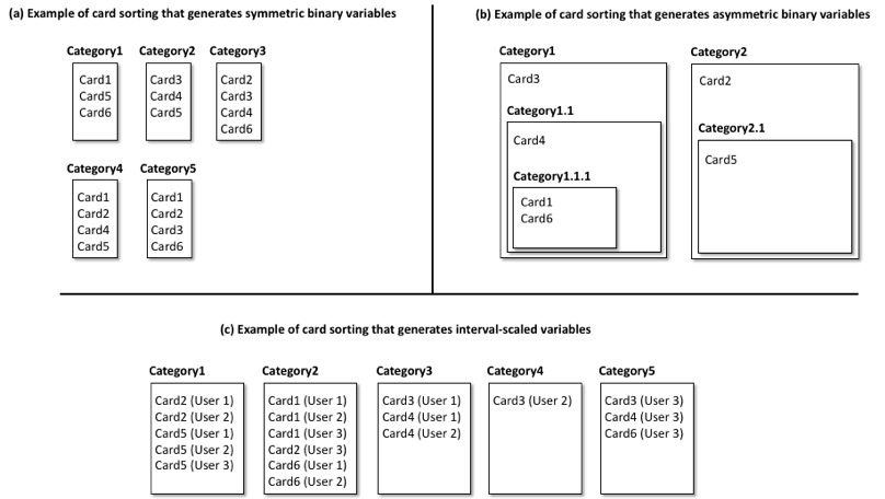
Figure 1. Different examples of card sorting (p = 6; n = 5) representing (a) an open unnormalized card sorting, (b) a nested-category card sorting, and (c) a normalized-category card sorting.

Table 1. Example of Symmetric Binary Variables (p = 6; n = 5)

	Card1	Card2	Card3	Card4	Card5	Card6
Category1	1	0	0	0	1	1
Category2	0	0	1	1	1	0
Category3	0	1	1	1	0	1
Category4	1	1	0	1	1	0
Category5	1	1	1	0	0	1

 

Table 2. Example of Asymmetric Binary Variables (p = 6; n = 5)

	Card1	Card2	Card3	Card4	Card5	Card6
Category1	1	0	1	1	0	1
Category1.1	1	0	0	1	0	1
Category1.1.1	1	0	0	0	0	1
Category2	0	1	0	0	1	0
Category2.1	0	0	0	0	1	0

Table 3. Example of Interval-Scaled Variables (p = 6; n = 5)

	Card1	Card2	Card3	Card4	Card5	Card6
Category1	0	2	0	0	3	0
Category2	3	1	0	0	0	2
Category3	0	0	1	2	0	0
Category4	0	0	1	0	0	0
Category5	0	0	1	1	0	1

Distance Analysis

A second step toward producing the dendrogram is the selection of the suitable distance method according to the type of the card-sorting data. As the dendrogram is based on a hierarchical clustering approach, it requires a distance or dissimilarity matrix in order to calculate pairwise distances among variables. There are several methods to obtain a distance matrix (Drost, 2018), and this mostly depend on the type of the data. In the case of card-sorting data, there are different distance metrics to apply:

• Lq metrics (also known as Minkowski family): The general formula of the Minkowski distance (d) among two variables (v₁ and v₂) of length n can be defined as the following:

     

This family includes the most used distance metrics such as Euclidean (q = 2) or Manhattan (q = 1), where the latter is also known as city-block, taxicab, or the snake metric. These metrics are based on minimizing the sums of dissimilarities. Euclidean distance, representing the straight-line distance among two points, is probably one of the most utilized, and it can be used with interval-scaled data but also with symmetric binary data (Kaufman & Rousseeuw, 2009), providing suitable results in both cases.

• • L₁ metrics: They are generally based on minimizing the average sums of dissimilarities, and include metrics such as Sorensen, Soergel, and Gower, to cite a few. One the most used is the Gower distance metric, which is more suitable for symmetric binary variables. It is based on calculating the average of partial dissimilarities among variables. This way, the general formula of the Gower distance (d) among two variables (v₁ and v₂) of length n and range R can be defined as the following:

       

• Inner Product metrics: They are based on the inner product theory of linear algebra, and they can be applied to asymmetric binary variables. This family include metrics such as Harmonic Mean, Cosine, Dice, Jaccard, and so on. The most utilized metric is the Jaccard distance, based on the Jaccard Coefficient (i.e., S-coefficient), which can be calculated as the ratio of the size of the intersection among two sets and the size of their union. More specifically, the Jaccard distance (d) among two variables (v₁ and v₂) of length n can be defined as the following:

     

More specific metrics can be customized when asymmetric weighted variables are considered. This might imply to assign specific weights or create customized contingency tables to calculate the Jaccard distance.

A simple example to understand the application of the principal metrics is provided. Let us consider the following six variables representing different categories in which users have attempted to classify cards. Specifically, the following representation is a working matrix where categories (six in this case) are represented in rows and cards (a total of 40) in columns. This is similar to the example described in Figure 1.a and Table 1, where card-sorting data indicate the relationship between each card and the categories where it has been classified. This is done by using symmetric binary values, where 1 indicates that a card was classified into a specific category and 0 the opposite.

Categories	Cards
fruits:	0 1 1 0 0 0 0 0 0 0 0 0 0 0 0 0 0 0 0 0 0 0 1 0 0 1 0 0 0 0 0 0 0 0 0 0 0 0 1 0
vegetables:	1 0 0 0 1 0 0 0 0 0 0 0 1 0 0 0 1 0 0 0 0 1 0 0 0 0 0 0 0 1 0 1 0 0 0 0 0 0 0 0
produce:	1 1 1 0 1 0 0 0 0 0 0 0 1 0 0 0 1 0 0 0 0 1 1 0 0 1 0 0 0 1 0 0 0 0 0 0 0 0 1 0
quick_energy:	0 0 0 1 0 0 1 1 0 0 0 1 0 1 0 0 0 0 0 1 0 0 0 1 1 0 0 1 0 1 1 1 0 0 1 0 1 0 0 0
dinners:	0 0 0 0 0 0 0 0 0 0 0 0 0 0 0 1 0 0 0 0 0 0 0 0 0 0 1 0 0 0 0 0 0 0 1 0 0 0 0 0
main_dishes:	0 0 0 0 0 0 0 0 0 0 0 0 0 0 0 1 0 0 0 0 0 0 0 0 0 0 1 0 0 0 0 0 0 0 1 0 0 0 0 0

Considering such categories, it is possible to calculate their distances or dissimilarities based on appropriate metrics for symmetric binary variables. This way, Lq metrics such as Euclidean, Manhattan, and Minkowski, and L₁ metrics such as Sorensen, Gower, and Soergel have been applied (see Table 4).

Table 4. Examples of Distance Calculations Based on the Previously Presented Categories

Distance among variables	Euclidean	Manhattan	Minkowski	Sorensen	Gower	Soergel
d(fruits, vegetables)	3,46	12,00	1,64	1,00	0,30	1,00
d(produce, quick_energy)	4,79	23,00	1,87	0,92	0,57	0,95
d(dinners, main_dishes)	0,00	0,00	0,00	0,00	0,00	0,00

As shown in Table 4, and taking into account the results of most metrics (Euclidean, Manhattan, Minkowski, and Gower), it can be concluded that the categories produce and quick_energy are strongly dissimilar (very distant) from each another, whereas fruits and vegetables can be considered as dissimilar, and dinners and main_dishes are strongly similar (closer). Note that similarity and dissimilarity in this context is related to the number of cards classified in each category, which implies that, for instance, dinners and main_dishes can be considered as similar categories as they classify the same cards (i.e., cards 16, 27, and 35, representing hamburger, pizza, and spaghetti, respectively, in this example).

In the case of multivariate methods, such as the hierarchical agglomerative clustering, metrics based on the minimization of sums or averages of dissimilarities (L_q and L₁ families including metrics such as Euclidean, Manhattan, Minkowski, and Gower) may result more robust than others based on the sums of squares (L₂ family including metrics such as Squared Euclidean, Pearson, Neyman, and so on), being also more consistent for larger sample sizes and less sensitive to outliers (Kaufman & Rousseeuw, 2009).

Clustering Analysis

Once the distance matrix has been calculated, the next step is to select the right linkage criterion for producing the dendrogram. In general, the hierarchical clustering can be implemented through a bottom-up (agglomerative) or top-down (divisive) approach. The agglomerative approach is the most commonly used, and it initially considers each variable as a single cluster. This way, the method attempts to successively merge pairs of clusters until all the clusters have been merged into a big one containing all the variables. The linkage criterion defines the way the distance among two clusters is calculated to decide the fusion of both. There exist different approaches to consider. The following are the most utilized:

• Centroid: Known as UPGMC (Unweighted Pair Group Method using Centroids), it is based on the between-cluster dissimilarity. This way, the dissimilarity between two clusters is calculated as the distance between their geometric centroids.
• Median: Known as WPGMC (Weighted Pair Group Method using Centroids), it is based on the cluster median. This way, the dissimilarity between two clusters is calculated as the median distance between the variables of one cluster and the variables of the other cluster.
• Mcquitty: Also known as WPGMA (Weighted Pair Group Method using Arithmetic Averages) or the simple-average method, it is based on the average distance. This way, the dissimilarity between two clusters is calculated as the average distance between the variables of one cluster and the variables of the other cluster.
• Complete-linkage: Also known as the furthest neighbor method, it is based on the minimum inter-similarity. This way, the dissimilarity between two clusters is calculated as the distance between the most distant two variables in each cluster.
• Single-linkage: Also known as the nearest neighbor method, it is based on the maximum inter-similarity. This way, the dissimilarity between two clusters is calculated as the distance between the closest two variables in each cluster.
• Ward: Also known as MISSQ (Minimization of the Increase of Sum of Squares), it is based on the minimum variance, trying to minimize the within-cluster sum of squares. In this sense, the dissimilarity between two clusters is calculated as the sum of squared deviations from the variables to the centroids.

All the linkages can be utilized and no specific restrictions have to be initially considered. However, analyzing the different linkage criteria according to the way they operate, Single and Complete linkages reduce the fitness to a single similarity between a pair of variables, which usually hinder to reflect the distribution of the variables in a cluster. This may lead to produce undesirable clusters. In addition, Single-linkage produces chaining effects when variables are close together, identifying long chain-like clusters. Complete-linkage overcomes this problem, but it is sensitive to outliers. On the other hand, Centroid and Median linkages may produce inversions, which occurs when two clusters being merged appear closer to each other than pairs of clusters merged earlier.

In general, Ward is the most common and utilized approach, and it can be used with both interval-scaled and symmetric binary variables. It minimizes the loss of information between the individual variables and the cluster centroid level. Previous studies have proved that, in a broad context, Ward behaves better than other linkage methods (Saraçli et al., 2013).

As for asymmetric binary data, Jaccard distance, together with the previously commented clustering linkages can be utilized. However, it is more recommendable to utilize monothetic approaches such as DIVCLUS-T (Chavent et al., 2007) or MONA (Kaufman & Rousseeuw, 2009).

Once the dendrogram has been produced, a final step consists in analyzing the goodness of the solution obtained. To this end, the Cophenetic Correlation Coefficient (CCC) can be used to analyze the goodness of a dendrogram (Saraçli et al., 2013). CCC can be defined as follows:

   

Where x(i,j) represents the ordinary Euclidean distance between variables i and j, t(i,j) represents the dendrogrammatic distance (i.e., the height of the node at which these two variables are first joined together) between the model points T_i and T_j, represents the average value of x(i,j) and represents the average value of t(i,j).

In brief, CCC describes the linear correlation between the dissimilarities of each pair of variables and their corresponding cophenetic distances. The cophenetic distances represent an intergroup dissimilarity measure of two variables that were merged in the same cluster. This method has been used in different domains to analyze whether a dendrogram represents an appropriate solution or not. This way, a high correlation (closer to 1) among the original distances and the cophenetic ones indicates a high goodness for a given dendrogram.

There exist other approaches intended to compare two different dendrograms in order to analyze which solution is the best suited. On the one hand, the Robinson-Foulds metric, also known as symmetric difference metric (Pattengale et al., 2007), can be used to calculate the topological distances between two dendrograms. This metric represents the number of branches in a given dendrogram with a combination of variables that exist in it but not in any subtree of the compared dendrogram plus the same computation on the other way round. This way, two dendrograms can be considered similar if they are isomorphic and their isomorphism preserves the labeling. On the other hand, the Baker-Hubert Gamma index (Desgraupes, 2013) can be used to obtain the correlation among two dendrograms. This index provides a concordance measure that indicates that two dendrograms are concordant if the values classify in the same order in both dendrograms. As well as CCC, Gamma index provides values between -1 and 1. Values closer to 0 indicate that two dendrograms are not statistically similar.

Results

The following sections discuss the results for data characterization, distance analysis, and clustering analysis.

Data Characterization

In order to implement the theories addressed in the previous section, the dataset published on the Cardsorting.net website (Cardsorting.net, 2017) as part of a tutorial (Blanchard et al., 2017) has been utilized. This is a publicly available dataset representing the classification of food items into different categories. The dataset represents an open and single card sorting, where 24 participants attempted to classify 40 cards (p = 40), each one into a single category. Participants created a total of 240 categories (n = 240). Raw data utilized represent categories as they were created by the participants, with no normalization process achieved. This way, card-sorting data indicate the relationship between each card and the categories where it was classified by using symmetric binary values, where 1 indicates that a card was classified into a specific category and 0 the opposite.

Distance Analysis

Once the raw data have been characterized, a first analysis consists of utilizing the dataset to compare different distance methods to see how they correlate. Figure 2 shows the correlation of 36 different distance methods belonging to different families, including those commented in the “Method” section. Correlation is based on Spearman correlation coefficients at 95%. This way, the small circles denotate different correlation degrees (from -1 to 1) as depicted by the legend at the bottom. Only significant correlations (p-value < 0.05) are shown.

As depicted in Figure 2, different strong correlations blocks can be found. On the one hand, there is a strong correlation among distance methods belonging to the same or similar families such as Inner Product (Harmonic Mean, Inner Product, and Cosine) and Intersection (Intersection, Ruzicka). Also, other correlations can be found in methods belonging to Intersection (Non-Intersection, Tanimoto, Motyka, and Czekanowski), Inner Product (Dice and Jaccard) and L₁ (Sorensen and Soergel) families. On the other hand, another correlation block can be found in methods belonging to Squared L₂ (Pearson, Neyman, Squared Euclidean, etc.), Combinations (AVg, Kumar-Johnson, etc.), Shannon’s Entropy (Jensen Difference, Jeffreys, etc.), L₁ (Lorentzian, Canberra, and Gower), and L_q (Euclidean and Manhattan) families.

These results indicate that some distance matrices, obtained from the application of the different distance methods, seem highly correlated, denoting that the selection of any of those methods would provide similar results. In this case, as the data comprise symmetric binary variables, it is possible to utilize Euclidean (general purpose) or Gower (more specific for binary variables), which are highly correlated in one of the correlation blocks analyzed (i.e., the largest one at the bottom).

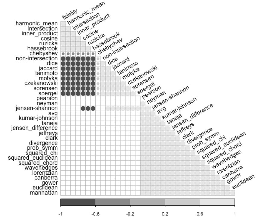
Figure 2. Spearman correlation coefficients obtained for the 36 distance methods compared. Only significant correlations at p-value < 0.05 are shown.

Clustering Analysis

A second analysis consists in calculating the Cophenetic Correlation Coefficients of the dendrograms generated through all the distance methods (a total of 36) and the linkage criteria (a total of six) previously analyzed. This way, Figure 3 shows the Cophenetic Correlation Coefficient for the 216 dendrograms generated.

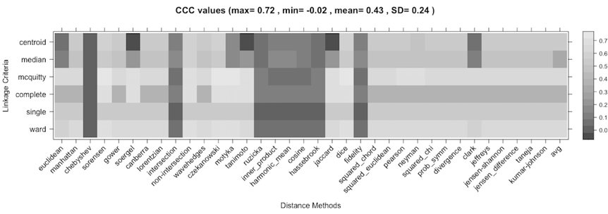
Figure 3. Cophenetic Correlation Coefficients for the 216 dendrograms obtained from the combinations of 36 distance methods and six linkage criteria.

As shown in Figure 3, there are some combinations obtaining high CCC values. In fact, Mcquitty linkage method combined with Sorensen, Czekanowski, Motyka, and Dice distance methods obtain the best CCC values (0.718). In addition, the classical combination of the Ward linkage with the Euclidean distance method provides a medium-high CCC value (0.6), similar to Gower using the same linkage method (0.62). According to the results obtained, all these solutions can be compared in several ways.

A first approach is to use the Robinson-Foulds metric. This provides a distance metric, indicating that the lower distance the similar two dendrogram are in terms of topological distance. Figure 4 shows the distances among the dendrograms with higher CCC values, including Euclidean and Gower distance methods with Ward linkage.

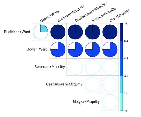
Figure 4. Distances among pairwise dendrogram comparisons. Higher values indicate more topological distance among dendrograms.

As shown in Figure 4, the Mcquitty linkage in combination with the three selected distance methods (Sorensen, Czekanowski, and Motyka) are the most similar in terms of topological distance, having a distance of 0 among them. On the other hand, Ward linkage combined with Euclidean and Gower distance methods provide also similar dendrograms (having a distance of 2). On the contrary, a comparison between dendrograms featuring Ward and Mcquitty linkages provides the higher distances (i.e., more dissimilar dendrograms in terms of topological distance).

Baker-Hubert Gamma index can be utilized to compare the similarity (association) among two dendrograms. Such index provides the rank correlation between the stages at which pairs of variables combine in each of the two dendrograms. This measure is not affected by the height of a branch. Instead, it is affected by the relative position of a branch compared with other branches. Baker-Hubert Gamma index provides a value that ranges from -1 to 1. A value closer to 0 indicates that the two dendrograms are not statistically similar. Figure 5 shows the Baker-Hubert Gamma indexes of the different configurations of dendrograms.

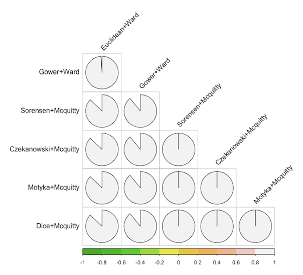
Figure 5. Baker-Hubert Gamma indexes of pairwise dendrogram comparisons. Values closer to 1 indicate higher correlation.

As shown in Figure 5, compared dendrograms have a high index over 0.87 in all cases, denoting a high statistical similarity. Analyzed apart, the groups of dendrogram based on Ward and Mcquitty linkages have the maximum statistical similarity, whereas pairwise correlations of mixed Ward and Mcquitty dendrograms produce correlations closer to 0.9. This implies that resulting dendrograms are similar in any case.

As a final step, dendrograms can be compared side by side in order to analyze relevant differences and the entanglement factor, which ranges from 0 (no entanglement) to 1 (full entanglement) indicating the quality of the alignment of the two dendrograms. In general, a lower entanglement coefficient corresponds to a better alignment.

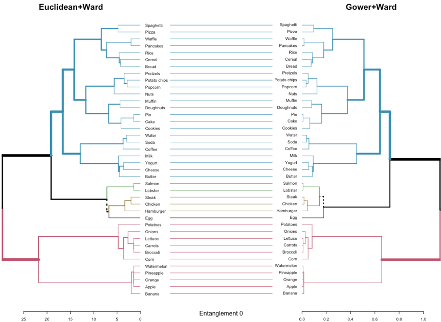
Figure 6. Dendrograms produced with Euclidean and Gower distance methods and Ward clustering linkage are compared. Entanglement factor is also provided.

Figure 6 depicts the comparison of two dendrograms generated with two different distance methods (i.e., Euclidean and Gower) and the Ward linkage criterion. As shown, unique branch fusions are highlighted with dashed lines, that is, branches containing a combination of variables that are not present in the other dendrogram. Connecting lines are colored to highlight sub-trees that are present in both dendrograms. Also, the width of the branches reflects the height.

As can be found in the related bibliography (Kaufman & Rousseeuw, 2009), a dendrogram is a clustering method where results are represented by a tree. This way, variables are grouped according to their similarity. The distance between merged clusters is monotone, increasing with the level of the merger. This way, the height of each node is proportional to the value of the intergroup dissimilarity between its branches.

As shown in Figure 6, both distance methods produce dendrograms very similar with minimal topological variations (dashed lines), which is also denoted by the low entanglement factor (0). Heights are, however, very different from one dendrogram to another. While Gower+Ward configuration promptly produces clusters with a lower height, Euclidean+Ward produce clusters with larger heights. It is worth mentioning that obtaining two trees with horizontal connecting lines does not imply that these dendrograms are identical (or even very similar in terms of topological structure). In this sense, the aforementioned correlation analyses are more accurate for decision-making.

Figure 7 shows the comparison of Euclidean+Ward and Sorensen+Mcquitty dendrograms. In this case, the two dendrograms include more topological and height-based differences, as it can be identified by the dashed lines, the connecting lines, and the entanglement factor (0.15). This corroborates, to some extent, the differences previously commented among Ward and Mcquitty linkages, which produce different clusters with different heights. In general, any compared configuration of Ward and Mcquitty linkages produce dendrograms with similar differences and entanglement.

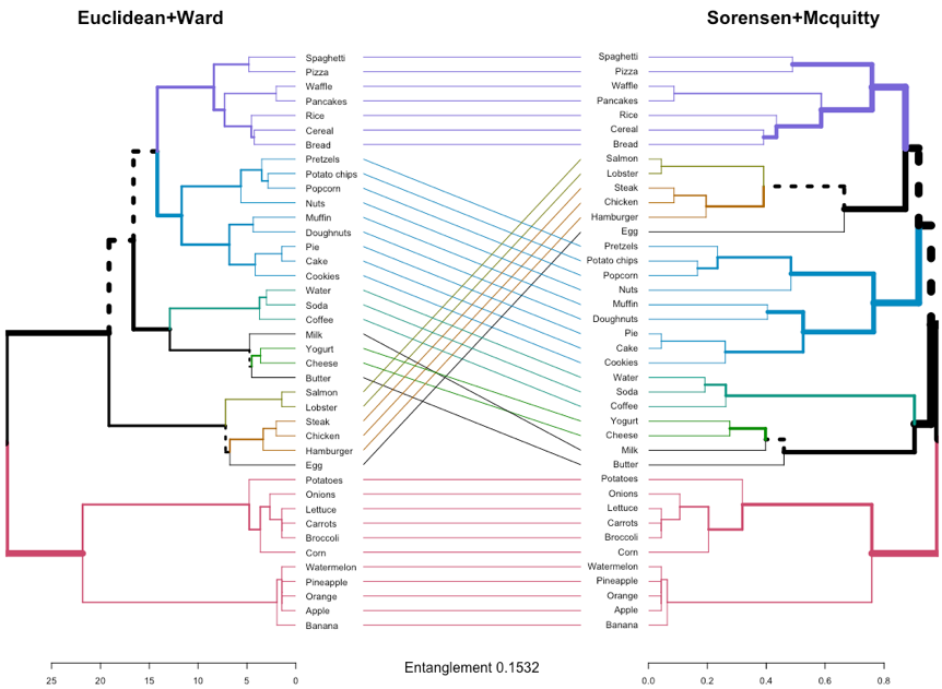
Figure 7. Dendrograms produced with Euclidean+Ward and Sorensen+Mcquitty configurations are compared. Entanglement factor is also provided.

Figure 8 shows the comparison of Sorensen+Mcquitty and Czekanowski+Mcquitty dendrograms. In this case, the two dendrograms are identical (i.e., all branches have the same color in both dendrograms) with a perfect entanglement. In general, any compared configuration of Mcquitty linkage with different distance methods produce similar results and identical dendrograms, corroborating the correlations previously analyzed.

In general, all the compared dendrograms are similar in terms of the conceptual clusters created that, in this case, are related to the classification of food items. However, topological and statistical differences exist in terms of the distance method and the linkage criterion applied, obtaining different topologies, branches, and heights. For instance, for a k = 11 solution, 7.17, 0.17, 0.58, 0.58, 0.79, and 0.58 height values are obtained for Euclidean+Ward, Gower+Ward, Sorensen+Mcquitty, Czekanowski+Mcquitty, Motyka+Mcquitty, and Dice+Mcquitty dendrograms, respectively. This indicates that Euclidean distance with Ward linkage produces the largest heights, whereas Gower+Ward combination produces the lowest ones. On the other hand, Mcquitty linkage produces similar heights using Sorensen, Czekanowski, Motyka, and Dice distance methods. The height value is useful to analyze how similar or not are two variables, but also to see the point of fusion of both two. Specifically, the higher the height of the fusion the less similar the variables are. As observed, this mostly depends on the distance method and the linkage criterion. For instance, a wrong decision would have been selecting Euclidean+Centroid configuration, which obtains a rather low CCC value of 0.070, a Robinson-Foulds distance of 36-38 compared with the rest of analyzed solutions and thus producing a rather different dendrogram with misleading conceptual classifications and an entanglement factor (compared with Euclidean+Ward configuration) of 0.46.

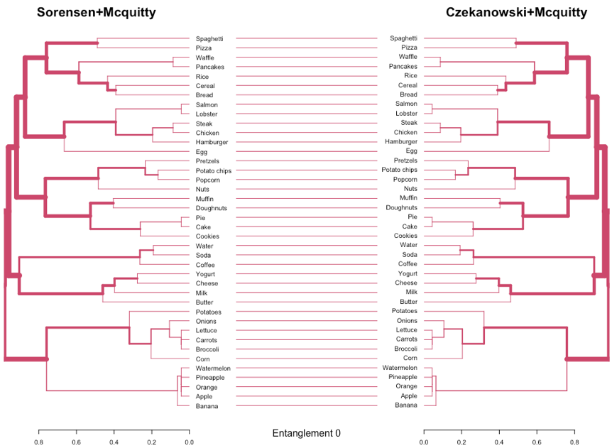
Figure 8. Dendrograms produced with Sorensen+Mcquitty and Czekanowski+Mcquitty configurations are compared. Entanglement factor is also provided.

Conclusion

Card sorting is one of the most utilized techniques in information architecture (Wood & Wood, 2008) and user experience. It represents a useful technique to understand a user’s mental model, being cost-effective and easy to implement, which makes it an essential technique for web-based development (Macías, 2008; Macías & Castells, 2001a, 2001b, 2001c). However, in a second phase, results obtained from card sorts should be properly analyzed. In fact, the quantitative analysis of card-sorting data is a necessary but complex step toward the suitable interpretation of results for decision-making.

Dendrograms have become one the most popular representations for the quantitative analysis of card-sorting data. Dendrograms are usually based on a hierarchical agglomerative clustering approach, where different parameters are involved and should be properly configured in order to obtain meaningful results. To this end, the characterization of raw data, the selection of an appropriate distance method and linkage criterion, and the evaluation of goodness indicators are essential in order to obtain reliable results for a suitable decision-making.

This paper is an attempt to analyze how such issues have an impact in the generation of suitable dendrograms for the quantitative analysis of resulting card-sorting data, providing different clues and indications of the different configurations according to the initial raw data available. Different comparative configurations, utilizing goodness indicators, have been provided, using a dataset containing a representative number of both variables and observations. Although, for the sake of brevity, only one specific dataset has been utilized to illustrate the proposed method, analysis and keystones provided here are widely generalizable to other domains and card-sorting datasets. In fact, different indications have been provided for different data types (binary and interval-scaled) that can be considered as representative of most resulting card-sorting data.

Tips for Usability Practitioners

This paper presents a set of clues intended to produce and analyze suitable dendrograms for the quantitative analysis of card-sorting data. In this sense, the principal tips to consider for usability practitioners are mostly related to the characterization of raw data, the selection of a proper distance method and linkage criterion, and the analysis of goodness indicators to compare different proposed solutions. A summary of the most important issues is presented in Table 5. Principal tips for practitioners are the following:

• Take your time in analyzing and characterizing raw data, identifying variables (p value), observations (n value), and the type (interval-scaled, symmetric, or asymmetric binary) of the data. As a general rule, interval-scaled variables come from aggregated binary values when category normalization has been accomplished. Otherwise, it is expected to have symmetric (single-category classification) or asymmetric (nested-category classification) binary variables. It is convenient to utilize working matrices (as those presented in the “Data Characterization” section) in order to represent and simplify card-category relationships that will be used later on for further analysis.
• Utilize the right distance method according to the type of the (card-sorting) variables. In general, Euclidean distance works fine with interval-scaled and symmetric binary variables. However, Gower distance can be also utilized with symmetric binary variables. For asymmetric binary variables, it is advisable to utilize Jaccard distance.
• Consider analyzing different linkage (and even distance) methods, using goodness indicators such as CCC, Robinson-Foulds, and Baker-Hubert Gamma index in order to observe which dendrogram fits better considering also the conceptual clusters obtained. A useful approach is to represent pairs of dendrograms together with the corresponding entanglement and observe the heights of both two. Also, the height value at which each pair of variables are joined or combined in a dendrogram are useful to analyze the similarity among them. In general, a lower height in the combination of two variables represents a closer relationship among them.
• Choose the right analysis according to the type of the data. As a general rule, Euclidean distance method and Ward linkage criterion comprise a suitable configuration in order to represent dendrograms for most card-sorting data, as long as the data contain interval-scaled or symmetric binary values. For the specific case of asymmetric binary values, it is better to utilize Jaccard distance or monothetic algorithms such as DIVCLUS-T or MONA. Another choice is to utilize Factor Analysis (Capra, 2005) instead of dendrograms. However, special consideration should be taken to prevent singularity problems due to linear dependences among variables.

Table 5. Summary Table with Key Issues to Represent Suitable Dendrograms

Card sorting data type	Recommended distance method	Recommended linkage criterion	Observation
Interval-scaled	Euclidean	Ward	Usually, data coming from aggregated binary values with category normalization
Symmetric binary	Euclidean or Gower	Ward	Usually, data coming from unnormalized-category card sorts
Asymmetric binary	Jaccard	Further analysis and comparison (using goodness indicators) among different linkage criteria is recommended	Usually, data coming from nested-category card sorts. In this case, it is advisable to utilize monothetic algorithms such as DIVCLUS-T or MONA

Note: Goodness indicators should be considered, anyway, to obtain the most suitable solution.

Acknowledgements

This work was partially supported by the Spanish Government (grant number RTI2018-095255-B-I00) and the Madrid Research Council (grant number P2018/TCS-4314).

References

Albert, W., & Tullis, T. (2013). Measuring the user experience: Collecting, analyzing, and presenting usability metrics. Morgan Kaufmann.

Blanchard, S. J., Aloise, D., & DeSarbo, W. S. (2017). Extracting summary piles from sorting task data. Journal of Marketing Research, 54(3), 398–414.

Borges, C. R., & Macías, J. A. (2010, June 19-23). Feasible database querying using a visual end-user approach. Proceedings of ACM SIGCHI Symposium on Engineering Interactive Computing Systems – EICS’10 (pp. 187–192). Berlin, Germany: ACM.

Capra, M. G. (2005, September). Factor analysis of card sort data: An alternative to hierarchical cluster analysis. Proceedings of the Human Factors and Ergonomics Society Annual Meeting (Vol. 49, No. 5, pp. 691–695). Los Angeles, CA: SAGE Publications.

Cardsorting.net (2017). Dataset based on the classification of food items. SumPi Tutorial. Retrieved from http://cardsorting.net/tutorials/sumpi.html

Cayola, L., & Macías, J. A. (2018). Systematic guidance on usability methods in user-centered software development. Information and Software Technology, 97, 163–175.

Chaparro, B. S., Hinkle, V. D., & Riley, S. K. (2008). The usability of computerized card sorting: A comparison of three applications by researchers and end users. Journal of Usability Studies, 4(1), 31–48.

Chavent, M., Lechevallier, Y., & Briant, O. (2007). DIVCLUS-T: A monothetic divisive hierarchical clustering method. Computational Statistics & Data Analysis, 52(2), 687–701.

Desgraupes, B. (2013). Clustering indices. University of Paris Ouest-Lab Modal’X, 1, 34. Retrieved from https://cran.r-project.org/web/packages/clusterCrit/vignettes/clusterCrit.pdf

Drost, H. G. (2018). Philentropy: Information theory and distance quantification with R. Journal of Open Source Software, 3(26), 765.

Hastie, T., Tibshirani, R., & Friedman, J. (2017). The elements of statistical learning: Data mining, inference, and prediction. Springer.

Hudson, W. (2014). Card Sorting. The encyclopedia of human-computer interaction. interaction-design. Retrieved from https://www.interaction-design.org/literature/book/the-encyclopedia-of-human-computer-interaction-2nd-ed/card-sorting

Kaufman, L., & Rousseeuw, P. J. (2009). Finding groups in data: An introduction to cluster analysis. John Wiley & Sons.

Macías, J. A. (2008). Intelligent assistance in authoring dynamically generated web interfaces. World Wide Web, 11(2), 253–286.

Macías, J. A. (2012). Enhancing interaction design on the semantic web: A case study. IEEE Transactions on Systems, Man, and Cybernetics, Part C (Applications and Reviews), 42(6),

Macías, J. A., & Castells, P. (2001a, March 31-April 5). A generic presentation modeling system for adaptive web-based instructional applications. Proceedings of Human Factors in Computing Systems – CHI’01 (pp. 349–350). Seattle, USA: ACM.

Macías, J. A., & Castells, P. (2001b, August 5-10). Adaptive hypermedia presentation modeling for domain ontologies. Proceedings of International Conference on Human-Computer Interaction – HCII’2001 (pp. 710–714). New Orleans, USA: Lawrence Erlbaum Associates.

Macías, J. A., & Castells, P. (2001c). Interactive design of adaptive courses. In M. Ortega & J. Bravo (Eds.), Computers and Education—Towards an Interconnected Society (pp. 235-242). Kluwer Academic Publishers.

Macías, J. A., & Castells, P. (2002, July 10-12). Tailoring dynamic ontology-driven web documents by demonstration. Proceedings of International Conference on Information Visualisation – IV’02 (pp. 535–540). Los Alamitos, USA: IEEE.

Macías, J. A., Saltiveri, A. G., & Andrés, P. M. L. (2009). New Trends on Human-Computer Interaction: Research, Development, New Tools and Methods. Springer.

Pattengale, N. D., Gottlieb, E. J., & Moret, B. M. (2007). Efficiently computing the Robinson-Foulds metric. Journal of Computational Biology, 14(6), 724–735.

Paea, S., & Baird, R. (2018). Information Architecture (IA): Using multidimensional scaling (MDS) and K-Means clustering algorithm for analysis of card sorting data. Journal of Usability Studies, 13(3), 138–157.

Paul, C. L. (2008). A modified delphi approach to a new card sorting methodology. Journal of Usability studies, 4(1), 7–30.

Paul, C. L. (2014). Analyzing Card-Sorting Data Using Graph Visualization. Journal of Usability Studies, 9(3). 87–104.

Pawliczek, P., & Dzwinel, W. (2013). Interactive data mining by using multidimensional scaling. Procedia Computer Science, 18, 40–49.

Rojas, L. A., & Macías, J. A. (2019). Toward collisions produced in requirements rankings: A qualitative approach and experimental study. Journal of Systems and Software, 158, 110417.

Rosenfeld, L., & Morville, P. (2002). Information architecture for the world wide web. O’Reilly Media, Inc.

Saraçli, S., Doğan, N., & Doğan, İ. (2013). Comparison of hierarchical cluster analysis methods by cophenetic correlation. Journal of Inequalities and Applications, 2013(1), 203.

Sauro, J., & Lewis, J. R. (2016). Quantifying the user experience: Practical statistics for user research. Morgan Kaufmann.

Spencer, D. (2009). Card sorting: Designing usable categories. Rosenfeld Media.

Veral, R., & Macías, J. A. (2019). Supporting user-perceived usability benchmarking through a developed quantitative metric. International Journal of Human-Computer Studies, 122, 184–195.

Wood, J. R., & Wood, L. E. (2008). Card sorting: Current practices and beyond. Journal of Usability Studies, 4(1), 1–6.

Published in: in Volume 16, Issue 2,